4.4 Trees

By composing together several transformations, we can get more complex and more controlled fractals.

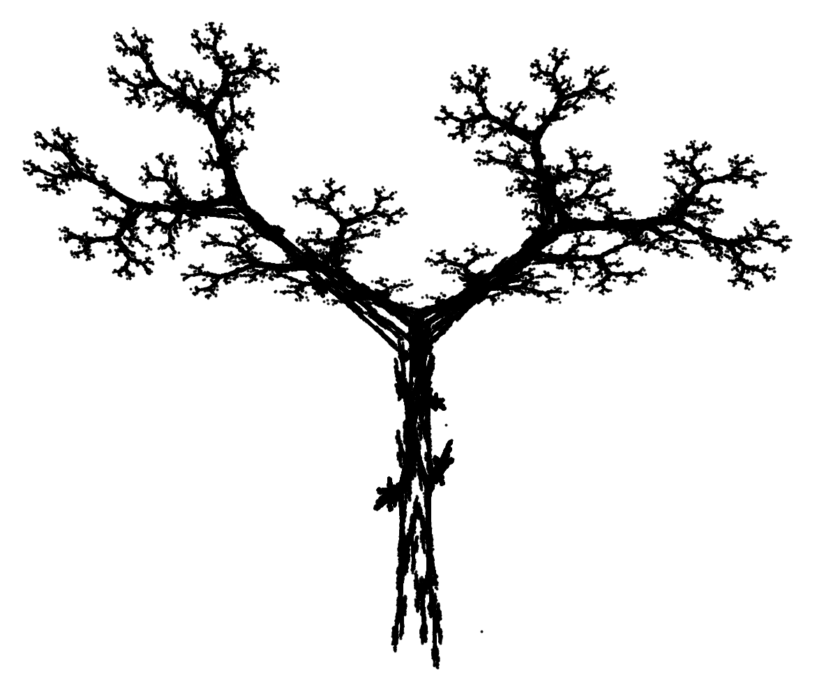
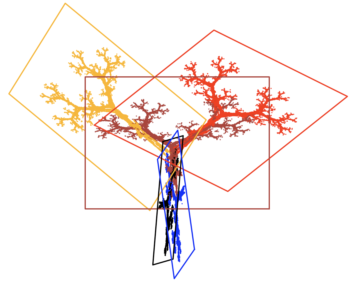
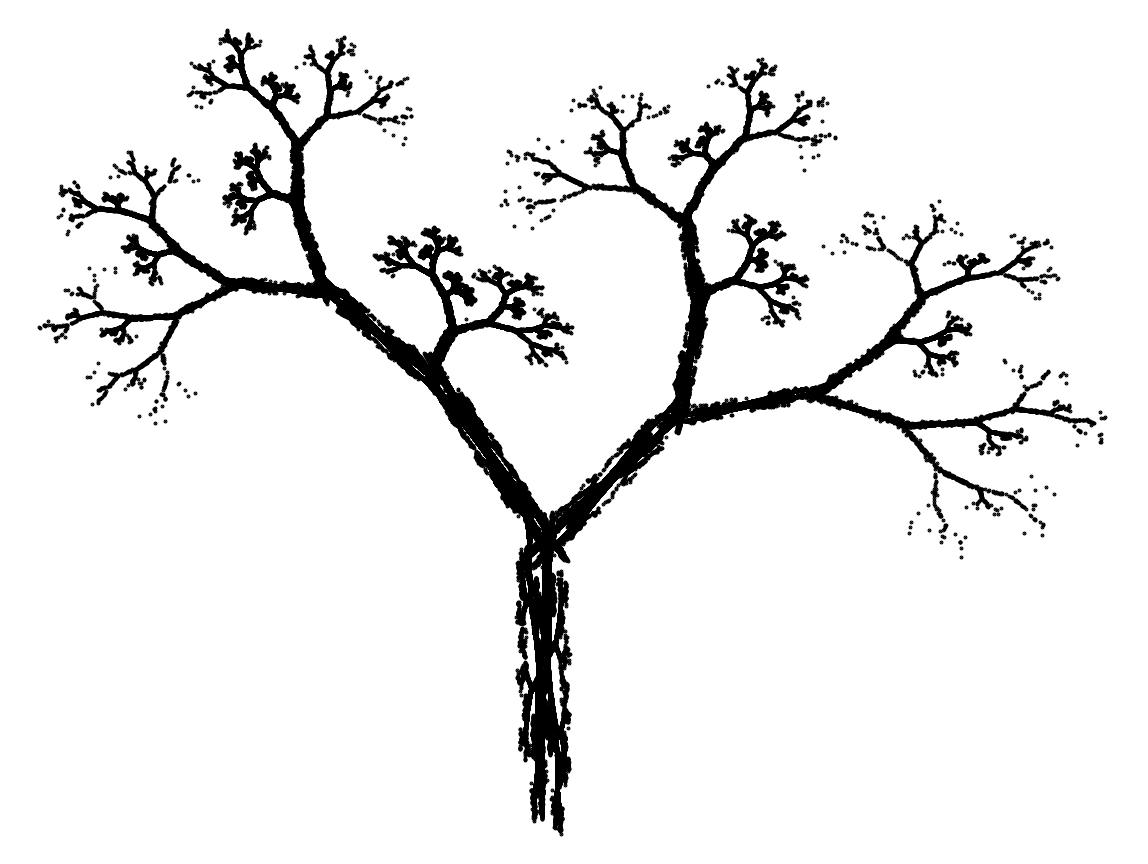
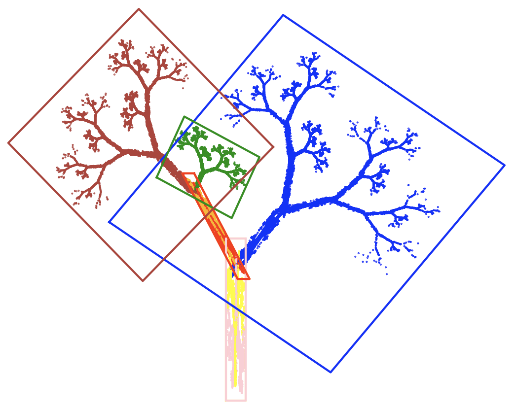
Below are examples of two fractals that look like trees. The first is composed of five and the second of seven transformations. Once you see the idea behind the tree structure, it’s easy to propose your own changes and extensions.

Transformations for the maple leaf. Color indicates the images resulting from successive transformations.

Each transformation is chosen with equal probability \(1/5\).

\[ f_1(x, y) = \begin{bmatrix} 0.195 & -0.488 & 0.4431 \\ 0.344 & 0.443 & 0.2452 \end{bmatrix} [x \ y \ 1]^T \] \[ f_2(x, y) = \begin{bmatrix} 0.462 & 0.414 & 0.2511 \\ -0.252 & 0.361 & 0.5692 \end{bmatrix} [x \ y \ 1]^T \] \[ f_3(x, y) = \begin{bmatrix} -0.637 & 0 & 0.8562 \\ 0 & 0.501 & 0.2512 \end{bmatrix} [x \ y \ 1]^T \] \[ f_4(x, y) = \begin{bmatrix} -0.035 & 0.07 & 0.4884 \\ -0.469 & 0.022 & 0.507 \end{bmatrix} [x \ y \ 1]^T \] \[ f_5(x, y) = \begin{bmatrix} -0.058 & -0.07 & 0.597 \\ 0.453 & -0.111 & 0.097 \end{bmatrix} [x \ y \ 1]^T \]

Some transformations overlap to create the effect of a thicker trunk or thicker branch.

Sections of this tree can be further lightened or darkened by changing the probability of choosing a transformation.

Transformations for the maple leaf. Color indicates the images resulting from successive transformations.

Each transformation is chosen with equal probability \(1/7\).

\[ f_1(x, y) = \begin{bmatrix} 0.05 & 0 & -0.06\\ 0 & 0.4 & -0.47 \end{bmatrix} [x \ y \ 1]^T \] \[ f_2(x, y) = \begin{bmatrix} -0.05 & 0 & -0.06 \\ 0 & -0.4 & -0.47 \end{bmatrix} [x \ y \ 1]^T \] \[ f_3(x, y) = \begin{bmatrix} 0.03 & -0.14 & -0.16 \\ 0 & 0.26 & -0.01 \end{bmatrix} [x \ y \ 1]^T \] \[ f_4(x, y) = \begin{bmatrix} -0.03 & 0.14 & -0.16 \\ 0 & -0.26 & -0.01 \end{bmatrix} [x \ y \ 1]^T \] \[ f_5(x, y) = \begin{bmatrix} 0.56 & 0.44 & 0.3 \\ -0.37 & 0.51 & 0.15 \end{bmatrix} [x \ y \ 1]^T \] \[ f_6(x, y) = \begin{bmatrix} 0.19 & 0.07 & -0.2 \\ -0.1 & 0.15 & 0.28 \end{bmatrix} [x \ y \ 1]^T \] \[ f_7(x, y) = \begin{bmatrix} -0.33 & -0.34 & -0.54 \\ -0.33 & 0.34 & 0.39 \end{bmatrix} [x \ y \ 1]^T \]