2.2 Fractal, that is fixed point
The highlight of this chapter will be the Banach fixed-point theorem and the relation of this theorem to fractals. We will start by showing the construction of some new exciting figures, such as Heighway dragon and Barnsley fern. Having satisfied the first curiosity, we will delve into the mathematical basis of these figures. For those who have studied mathematics, this can be a reminder of some concepts from mathematical analysis or topology. For those who have not studied mathematics, it may be an interesting look at how mathematicians formulate theorems.
2.2.1 Dragons and ferns
The first chapter left us with a method for constructing three fractals. Each of them could be made by repeating the steps over and over again:
Algorithm for constructing simple fractals.
- Take a shape.
- Copy it \(x\) times
- Scale it down by a factor of \(y\).
- Move the scaled copies around.
- Go back to step 2.
For Cantor dust, we copied \(x=2\) times and scaled down by a factor of \(y=3\). For the Sierpiński triangle, we copied \(x=3\) times, and scaled down by a factor of \(y=2\). For the Sierpiński carpet, we copied \(x=8\) times, and scaled down by a factor of \(y=3\).
It turns out that other different fractals can be created in a very similar way. And if we still allow rotations in addition to scaling and sliding, we get a very rich class of interesting figures. The combination of scaling, sliding, and rotation is such an important operation that it got its own name: affine transformation. An affine transformation turns line segments into line segments, straight lines into straight lines, and parallel lines into parallel lines. We will define it more formally in a few pages
In step 1 of the above algorithm, we choose any shape. But the more times we repeat step 3 of this algorithm, the smaller the selected figures become. In fact, the choice of this figure doesn’t matter, we might as well draw a triangle or an elephant or a small dot at the beginning. How is this possible? This will be the main conclusion of Banach fixed-point theorem.
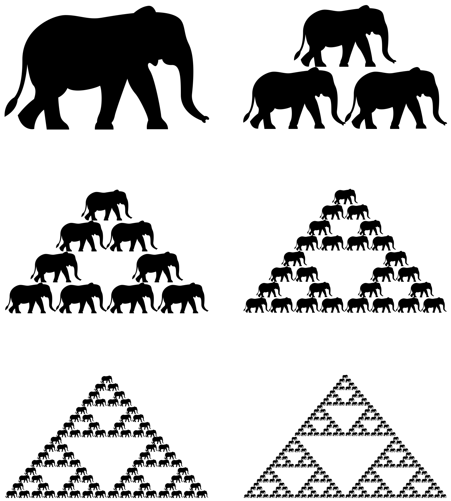
Let’s take a drawing of elephant. After six iterations, the elephant gets the size of a grain of sand anyway.
But first, let’s get to know three new fractals.
2.2.2 Sierpinski pentagon
We can repeat the trick with a triangle or square with any regular polygon, such as a pentagon.
Let’s copy the initial figure five times, then scale these copies down by a factor of \(\frac{3-\sqrt 5}2 \approx 0.382\), and then shift them to the corners of the pentagon so that the scaled figures meet the vertices. After repeating this procedure many times, we will obtain a figure called the Sierpiński pentagon.
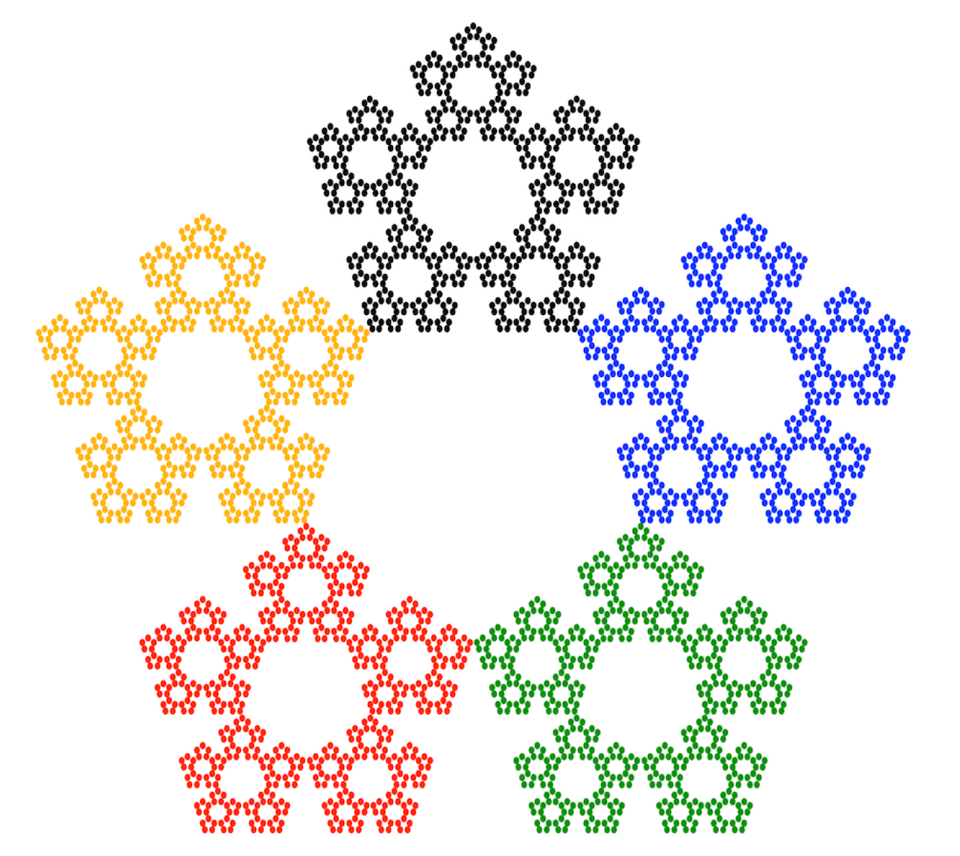
Sierpiński pentagon. The result of copying the input figure five times, scaling, and shifting these copies. Each of the five copies is marked with a different color.
But the real magic begins when we allow rotations in these transformations. Consider the following algorithm.
Algorithm for the construction of complex fractals.
- Take any shape.
- Copy it \(x\) times.
- Scale it down by a factor of \(y\).
- Rotate and/or shift the scaled copies.
- Go to step 2.
Let’s see how this algorithm works using a few interesting sets of transformations as an example.
2.2.3 Pythagoras tree
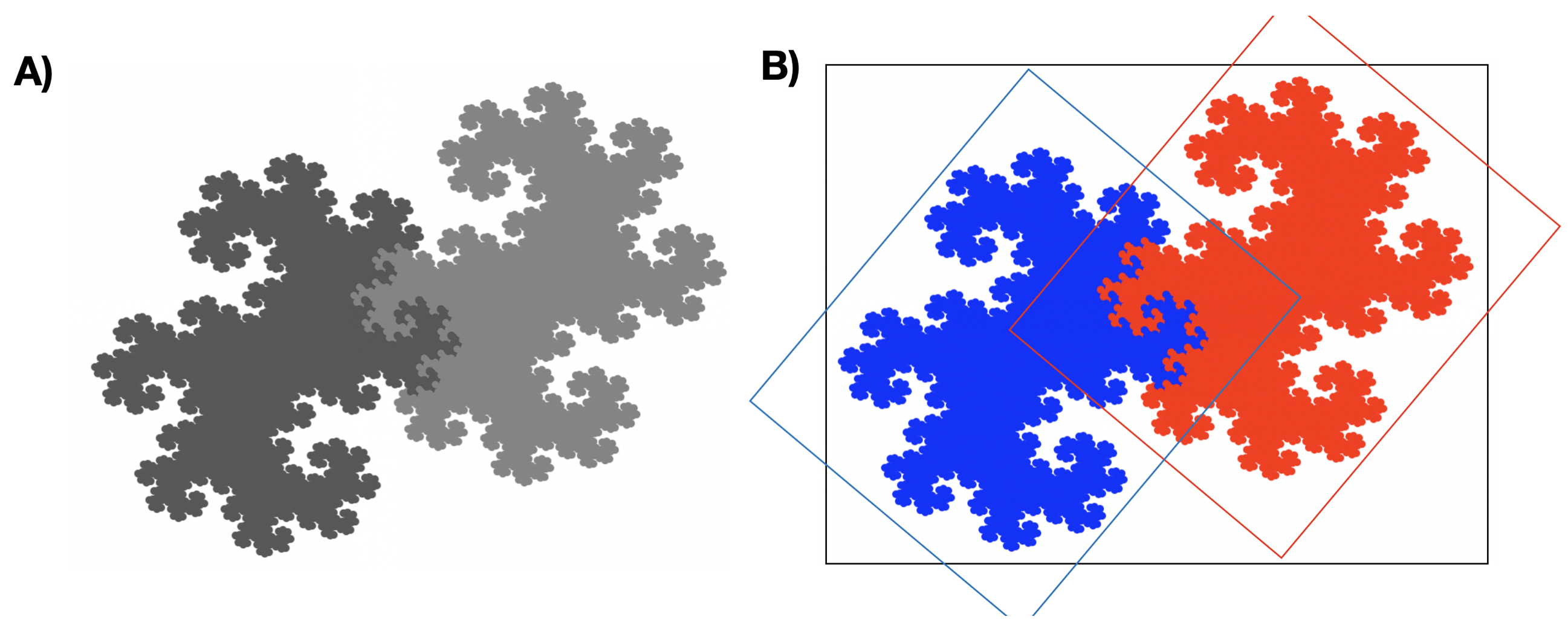
The construction of this fractal was described in 1942 by Albert Bosman. There are several different methods of constructing this figure. Below is a construction based on two transformations.
- Transformation 1: rotate the figure by \(45^{\circ}\) counterclockwise, then scale it by a factor of \(1/\sqrt{2}\).
- Transformation 2: rotate the figure by \(45^{\circ}\) clockwise, and then scale it by a factor of \(1/\sqrt{2}\).
The image below illustrates the fractal and shows the self-similarity resulting from composing transformations. The code to reproduce this fractal can be found at the end of the chapter.
Panel A shows a Pythagoras tree, and panel B illustrates the two transformations that make up the fractal. The image is scaled down by a factor of \(\sqrt{2}\) and rotated by 45 degrees. Each of the two replications is marked with a different color.
2.2.4 Heighway Dragon
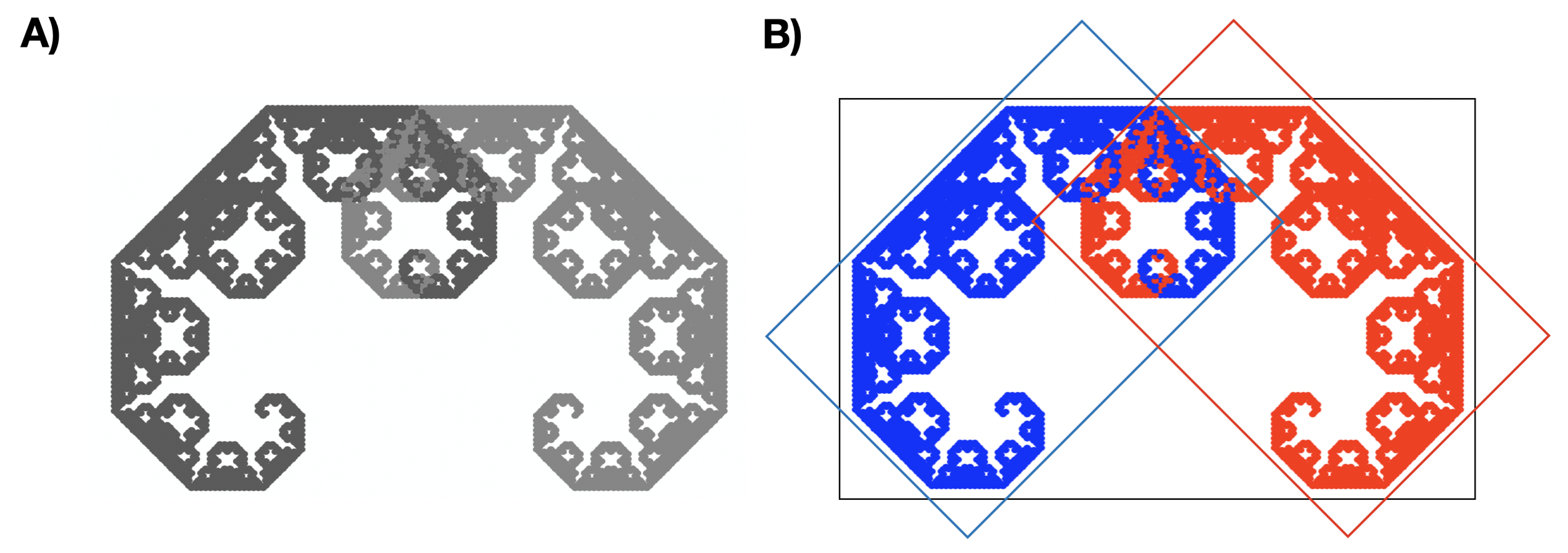
It turns out that a lot of interesting figures can be obtained using only two transformations. One such figure is the Heighway dragon, whose construction was first shown by NASA physicists John Heighway, Bruce Banks, and William Harter. The dragon is based on two transformations:
- Transformation 1: rotate the figure by \(45^{\circ}\) counterclockwise, then scale it by a factor of \(1/\sqrt 2\).
- Transformation 2: rotate the figure by \(45^{\circ}\) counterclockwise, then scale it by a factor of \(1/\sqrt 2\), and shift it by 1 along the horizontal axis.
The image below illustrates the dragon and both transformations. The code to reproduce this fractal can be found at the end of the chapter.
Panel A shows the Heighway dragon, and panel B illustrates the two transformations that make up the fractal. Each of the two replications is marked with a different color.
2.2.5 Barnsley fern
You can achieve a lot with two transformations, but what happens when you add more? Let’s see with the example of one of the most famous fractals – Barnsley fern. It was first described in 1993 by British mathematician Michael Barnsley, who studied fractals for their potential in fractal compression.
For ferns, we will need four transformations:
- Transformation 1 (left leaf): rotate the figure by \(10^{\circ}\) counterclockwise, then scale it by a factor of \((0.5; 0.3)\).
- Transformation 2 (right leaf): rotate the figure by\(15^{\circ}\) clockwise, then scale it by a factor of \((0.45; 0.25)\).
- Transformation 3 (top): rotate the figure by \(1^{\circ}\) clockwise, then scale it by a factor of \(0.9\), and shift it by \(0.01\) along the X axis.
- Transformation 4 (stem): scale the figure by a factor of \((0.25, 0)\).
The image below illustrates a fern and all four transformations. The code to reproduce this fractal can be found at the end of the chapter.
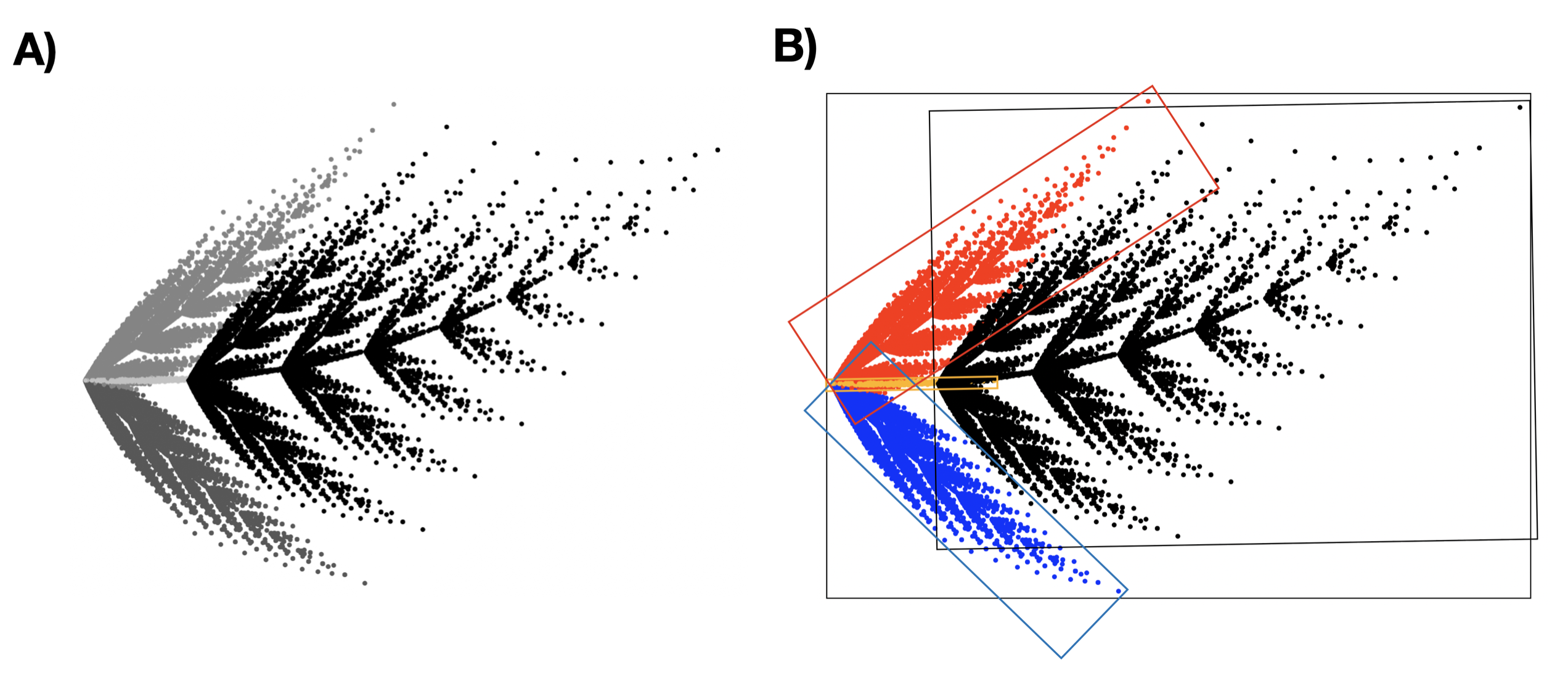
Panel A shows a Barnsley fern, and panel B illustrates the four transformations that make up the fractal. Each of the four replications is marked with a different color.