3.4 Examples in Python
3.4.1 The Sierpinski triangle once again
The following code reproduces the Sierpiński triangle construction presented in this chapter. In the triangle vector, we define the three vertices of the triangle, and in the point object we put the coordinates of the starting point for the fractal construction. We then move the point toward a random vertex in a loop.
- \(x' = x/2\), \(y' = y/2\) (left corner)
- \(x' = x/2 + \frac 12\), \(y' = y/2\) (right corner)
- \(x' = x/2 + \frac 14\), \(y' = y/2 + \frac{\sqrt{3}}2\) (upper corner)
import numpy as np
import matplotlib.pyplot as plt

# Number of steps of chaos game.
N = 200000
x_vec, y_vec, col_vec = [], [], []
# The coordinates of the vertices of the triangle.
triangle = [[0,0], [0.5, 2], [1.5,0.5]]
point = [0.1, 0]

# Randomly draw the number of the vertex in the direction of which we will move the point.
for i in range(N):
  ind = np.random.choice(range(3))
  point = np.multiply(np.add(point, triangle[ind]), 0.5)
  x_vec.append(point[0])
  y_vec.append(point[1])
  col_vec.append(ind)

# Draw a scatter plot from the visited points.
# Colors correspond to the drawn transformation.
plt.scatter(x_vec, y_vec, s=0.2, c = col_vec)
plt.axis('off')
plt.show()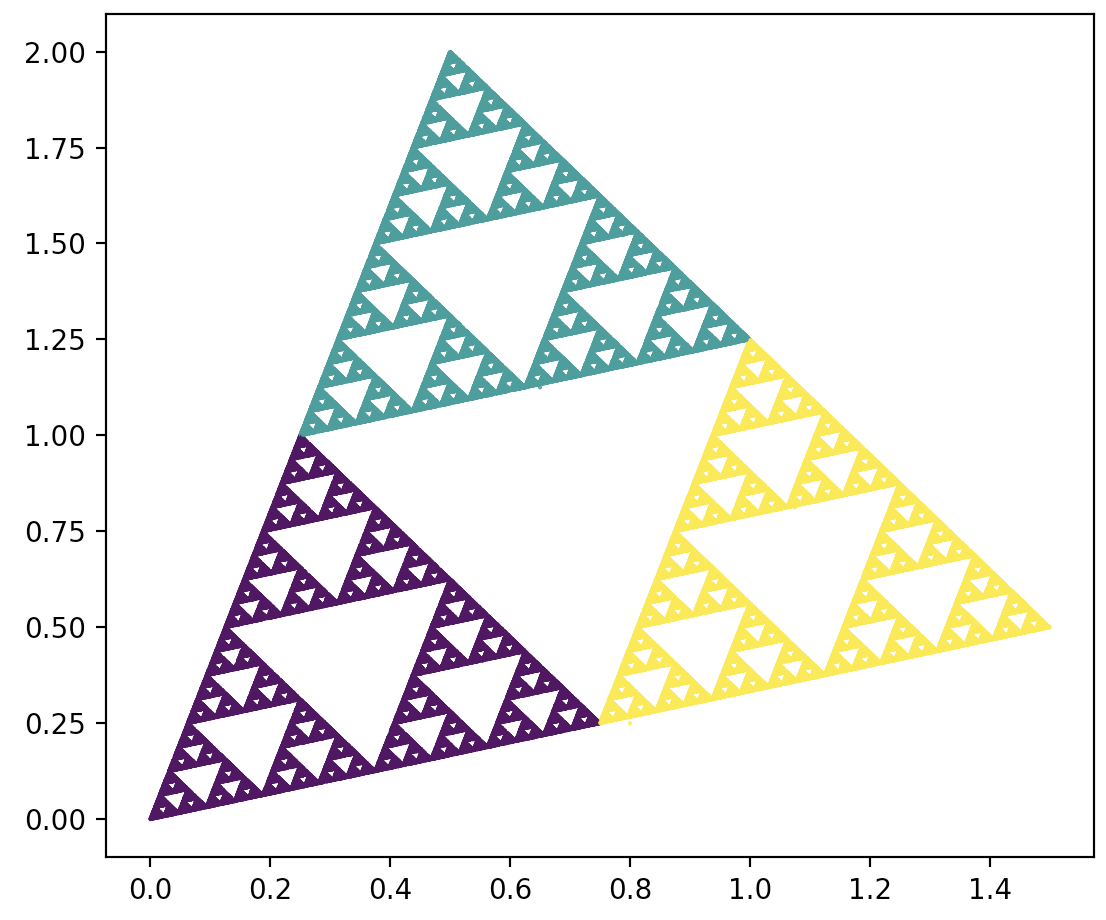
3.4.2 Barnsley fern
import numpy as np
import matplotlib.pyplot as plt

# Four transformations that make up a fern.
def trans1(x,y):
  return (0., 0.16*y)
def trans2(x,y):
  return (0.85*x + 0.04*y, -0.04*x + 0.85*y + 1.6)
def trans3(x,y):
  return (0.2*x - 0.26*y, 0.23*x + 0.22*y + 0.8)
def trans4(x,y):
  return (-0.15*x + 0.28*y, 0.26*x + 0.24*y + 0.44)

# List of transformations and vector with probabilities of drawing each transformation.
N, x, y = 200000, 0, 0
x_vec, y_vec, col_vec = [], [], []
trans = [trans1, trans2, trans3, trans4]
probs = [0.01, 0.79, 0.1, 0.1]

for i in range(N):
  # We draw one of the four transformations.
  ind = np.random.choice(range(len(trans)), p=probs)
  selected = trans[ind]
  x, y = selected(x,y)
  x_vec.append(x)
  y_vec.append(y)
  col_vec.append(ind)

plt.scatter(y_vec, x_vec, s=0.2, c=col_vec)
plt.show()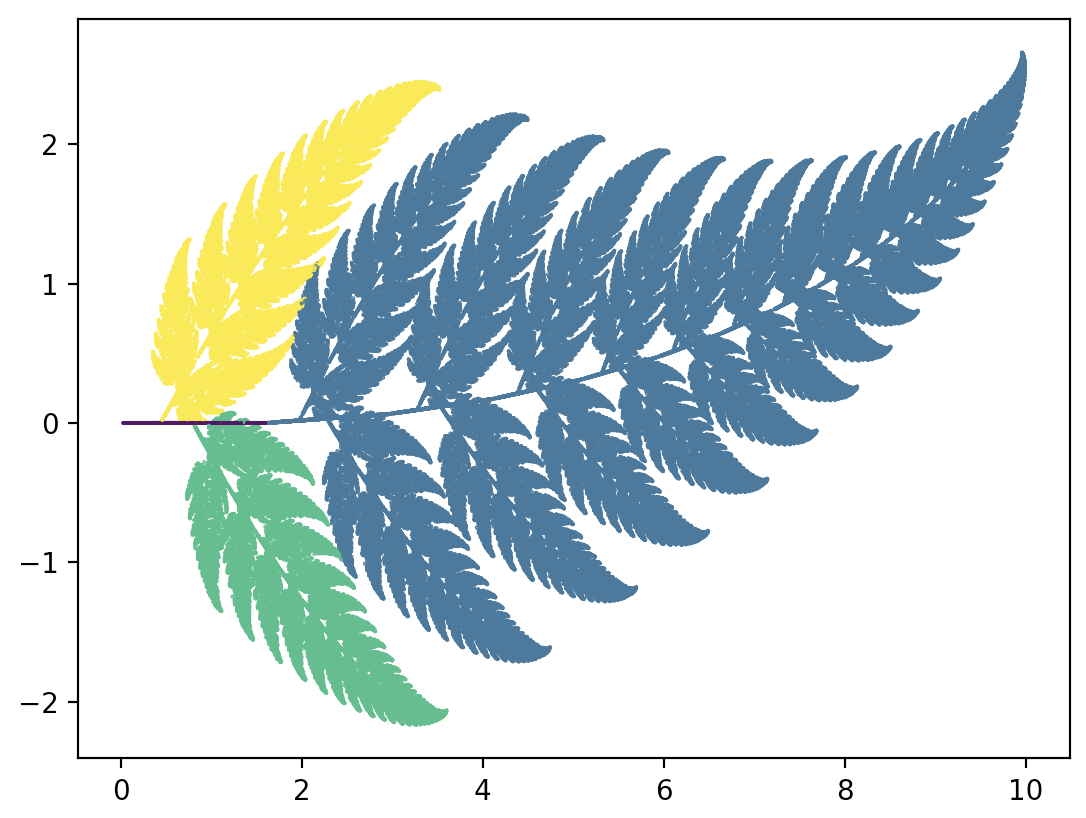
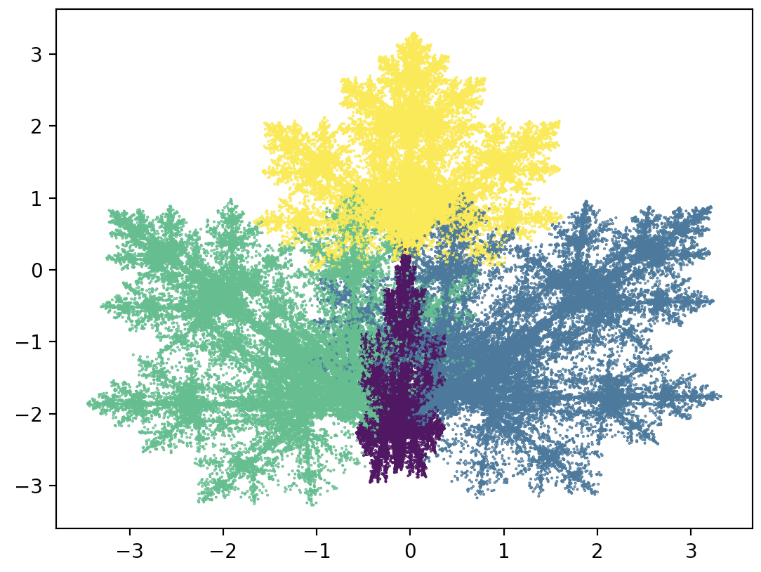
3.4.3 Maple leaf
import numpy as np
import matplotlib.pyplot as plt

def transform(x,y, affine):
  return(affine[0]*x + affine[1]*y + affine[2],
         affine[3]*x + affine[4]*y + affine[5])

N, x, y = 200000, 0, 0
x_vec, y_vec, col_vec = [], [], []
# List of transformations.
affines = [[0.14, 0.01, -0.08, 0.0, 0.51, -1.31],
  [0.43, 0.52, 1.49, -0.45, 0.5, -0.75],
  [0.45, -0.49, -1.62, 0.47, 0.47, -0.74],
  [0.49, 0.0, 0.02, 0.0, 0.51, 1.62]]
probs = [0.25, 0.25, 0.25, 0.25]

for i in range(N):
  # We randomly choose one of the four transformations.
  ind = np.random.choice(range(len(affines)), p=probs)
  x, y = transform(x,y, affines[ind])
  x_vec.append(x)
  y_vec.append(y)
  col_vec.append(ind)

plt.scatter(x_vec, y_vec, s=0.2, c=col_vec)
plt.show()