2.5 Examples in R

The examples presented in this chapter repeat the composition of three atomic transformations – shift, rescale and rotate. Below are the definitions of these three transformations. In these examples, x is a two-element vector.

# Move point x by delta.
shift = function(x, delta)  
  x + delta

# Scale point x times ratio.
scale = function(x, ratio) 
  x * ratio

# Rotate by alpha angle (in degrees).
rotate = function(x, alpha) { 
  sa = sin(pi * alpha / 180)
  ca = cos(pi * alpha / 180)
  x %*% matrix(c(ca, -sa, sa, ca), 2, 2, byrow = TRUE)
}

2.5.1 Sierpiński triangle

As we wrote at the beginning of this chapter, fractals can be built from ordinary dots, we do not need more sophisticated polygons. Let’s introduce it based on the Sierpiński triangle.

\[ y_1 = x * \left[\begin{smallmatrix} 0.5 & 0\\ 0 & 0.5 \end{smallmatrix}\right] \]

\[ y_2 = x * \left[\begin{smallmatrix} 0.5 & 0\\ 0 & 0.5 \end{smallmatrix}\right] + \left[\begin{smallmatrix} 0.5 \\ 0 \end{smallmatrix}\right] \]

\[ y_3 = x * \left[\begin{smallmatrix} 0.5 & 0\\ 0 & 0.5 \end{smallmatrix}\right] + \left[\begin{smallmatrix} 0.25 \\ \sqrt3/4 \end{smallmatrix}\right] \]

# The notation x |> scale(0.5) |> shift(0.2) in R denotes the 
# tail composite of these functions and is equivalent to the notation
# shift(scale(x, 0.5), 0.2). However, it is more readable.
sierpinski <- function(x, depth, col = "black") {
  if (depth > 1) {
    x1 = x |> scale(0.5) 
    sierpinski(x1, depth - 1, col = "blue")
    x2 = x |> scale(0.5) |> shift(c(0.5, 0)) 
    sierpinski(x2, depth - 1, col = "red")
    x3 = x |> scale(0.5) |> shift(c(0.25, 0.5)) 
    sierpinski(x3, depth - 1, col = "orange")
  } else {
    points(x[1], x[2], pch = 19, col = col, cex=0.3) 
  }
}

plot.new()
plot.window(xlim=c(0, 1), ylim=c(0,1), asp=1)
sierpinski(c(0,0), depth = 8)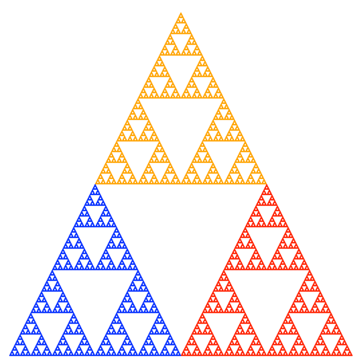

The result of executing the above instructions

2.5.2 Sierpiński pentagon

pentagon <- function(x, depth, color="black") {
  if (depth > 1) {
    x1 = x |> scale(0.382) 
    pentagon(x1, depth - 1, color = "blue")
    x2 = x |> scale(0.382) |> shift(c(0.618, 0)) 
    pentagon(x2, depth - 1, color = "red")
    x3 = x |> scale(0.382) |> shift(c(0.809, 0.588)) 
    pentagon(x3, depth - 1, color = "green")
    x4 = x |> scale(0.382) |> shift(c(0.309, 0.951)) 
    pentagon(x4, depth - 1, color = "orange")
    x5 = x |> scale(0.382) |> shift(c(-0.191, 0.588)) 
    pentagon(x5, depth - 1, color = "pink")
  } else 
    points(x[1], x[2], pch = 19, col = color, cex=0.5) 
}

plot.new()
plot.window(xlim=c(-0.5,1.5), ylim=c(-0.1,1.7), asp=1)
pentagon(c(0,0), depth = 6)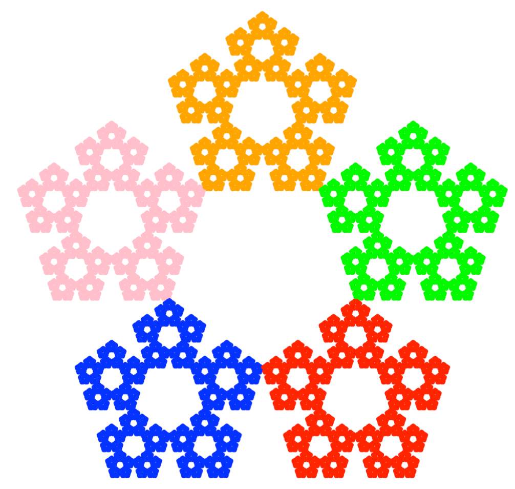

The result of executing the above instructions

2.5.3 Heighway’s Dragon

heighway <- function(x, depth, color="black") {
  if (depth > 1) {
    x1 = x|> rotate(45)|> scale(sqrt(0.5))|> shift(c(1,0)) 
    heighway(x1, depth-1, color="blue")
    x2 = x|> rotate(135)|> scale(sqrt(0.5)) 
    heighway(x2, depth-1, color="red")
  } else 
    points(x[1], x[2], pch=19, col=color, cex=0.5) 
}

plot.new()
plot.window(xlim=c(-1,2), ylim=c(-1.5,0.5), asp=1)
heighway(c(1,1), depth = 15)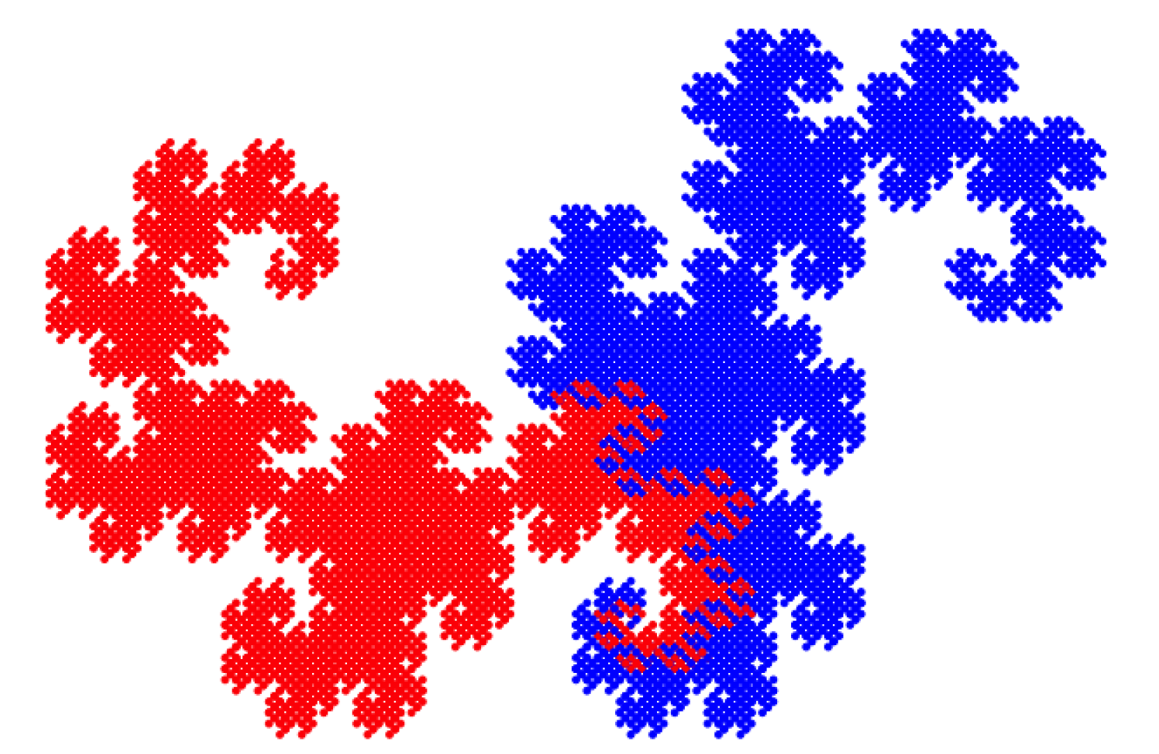

The result of executing the above instructions

2.5.4 Symmetric binary tree / Pythagoras’ tree

pitagoras = function(x, depth, color="black") {
  if (depth > 1) {
    x1 = x|> rotate(-45) |> scale(sqrt(0.5)) |> shift(c(0,1)) 
    pitagoras(x1, depth-1, color="blue")
    x2 = x|> rotate(45) |> scale(sqrt(0.5)) |> shift(c(0,1)) 
    pitagoras(x2, depth-1, color="red")
  } else 
    points(x[1], x[2], pch=19, col=color, cex=0.5) 
}

plot.new()
plot.window(xlim = c(-3,3), ylim = c(0,3), asp=1)
pitagoras(c(1,1), depth = 15)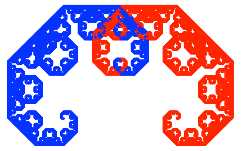

The result of executing the above instructions