1.5 Examples in R

Dear Reader, you can reproduce the described fractals on your computer. All you need is an installed R language interpreter, which can be freely downloaded and installed from CRAN. No prior knowledge of this language is necessary, although it would, of course, be helpful. Here is some information to help you understand this code.

1. The following examples use the basic graphics library for R, namely graphics. You don’t need to load it, as it is available immediately after starting R. The plot.new() function creates an empty graph. It is filled by using the polygon() function to draw filled polygons, here, a triangle and a square.
2. R is a language for mathematicians and statisticians, so most of the mathematical operations are available as soon as you start the console, like the sqrt() function needed to calculate the height of an equilateral triangle.
3. The R works natively on vectors, which means we can use arithmetic operators such as + or / for both numbers and vectors.
4. To make the code more readable, we use recursion, a situation in which a function calls itself. New functions are defined using the function keyword. The functions shown have a depth argument, specifying how many more times the function should call itself.

1.5.1 Cantor dust

Let’s start drawing fractals with Cantor dust. For this, we will use the recursive function dust, which takes four arguments: x, y – the location from which to draw the fractal, scale – information about the size of the fractal, and depth – the current nesting level of the fractal.

# Recursive function to draw dust. 
# If depth=1, it draws a line segment, 
# if depth>1 it draws two copies of Cantor dust side by side.
dust = function(x, y, scale, depth = 1) { 
  if (depth == 0) {
    lines(c(x, x + scale), c(y, y))
  } else {
    dust(x, y, scale/3, depth - 1)
    dust(x + scale*2/3, y, scale/3, depth - 1)
  }
}

# Clear the screen and start drawing dust.
plot.new() 
dust(0, 0, scale = 1, depth = 4)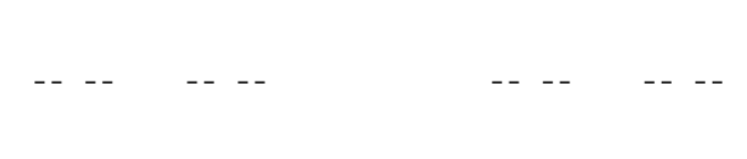

The result of executing the following instructions

1.5.2 Sierpinski triangle

It’s time for the iconic Sierpiński triangle. To draw it, we will use the recursive function sierpinski(), which takes four arguments: x, y – the location from which to draw the fractal, scale – information about the size of the fractal, and depth – the current nesting level of the fractal.

triangle <- function(x, y, scale) {
  polygon(x + scale*c(0, 1, 1/2), 
          y + scale*c(0, 0, sqrt(3)/2), col = "black")
}

# Recursive function to draw Sierpiński triangle. 
# If depth=1, we draw a triangle using the triangle() function, 
# if depth>1, we draw three triangles side by side.
sierpinski <- function(x, y, scale, depth = 1) { 
  if (depth == 0) {
    triangle(x, y, scale)
  } else {
    sierpinski(x, y, scale/2, depth-1)
    sierpinski(x+scale/2, y, scale/2, depth-1)
    sierpinski(x+scale/4, y+sqrt(3)*scale/4,scale/2,depth-1)
  }
}

plot.new()
sierpinski(0, 0, scale = 1, depth = 6)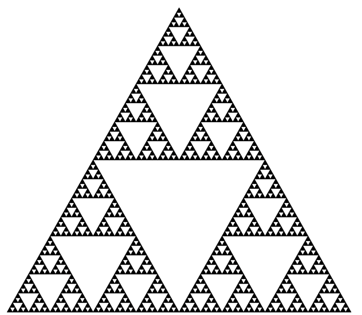

The result of executing the following instructions

1.5.3 Sierpinski carpet

The fractal structure proposed by Wacław Sierpiński can be repeated for other shapes.

# Recursive function to draw a carpet.
# Depending on the current depth, it either draws a square or, recursively calls itself eight times.
carpet = function(x, y, scale, depth = 1) { 
  if (depth == 1) {
    rect(x, y, x + scale, y + scale, col = "black")
  } else {
    carpet(x, y, scale/3, depth - 1)
    carpet(x+scale*1/3, y, scale/3, depth - 1)
    carpet(x+scale*2/3, y, scale/3, depth - 1)
    carpet(x, y+scale*1/3, scale/3, depth - 1)
    carpet(x+scale*2/3, y+scale*1/3, scale/3, depth - 1)
    carpet(x, y+scale*2/3, scale/3, depth - 1)
    carpet(x+scale*1/3, y+scale*2/3, scale/3, depth - 1)
    carpet(x+scale*2/3, y+scale*2/3, scale/3, depth - 1)  
  }
}

plot.new()
carpet(0, 0, scale = 1, depth = 4)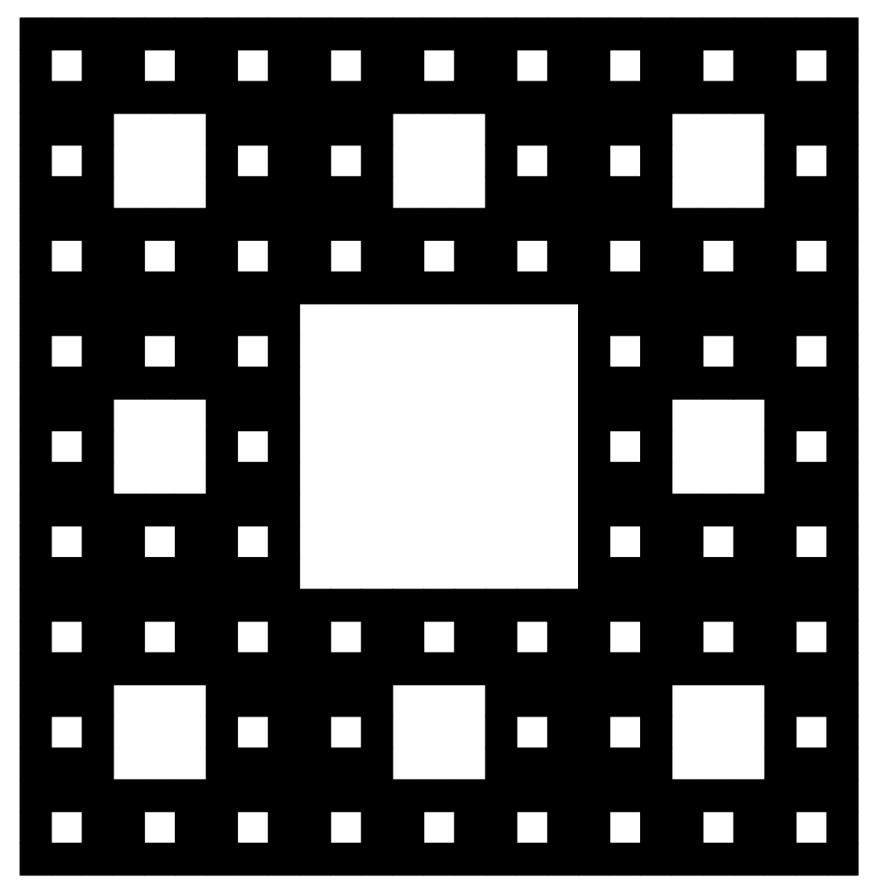

The result of executing the following instructions}