2.3 But why does it work?
The figures shown have a very interesting mathematical description. We present it below at the level of detail of the first years of mathematical studies. First, we will define some necessary concepts, based on which we can present the fixed-point theorem.
Usually, when thinking about figures and distances, we focus on a very classic plane with two axes and the common Euclidean distance. But for the upcoming theorem, we need to look at some ideas a bit more abstractly.
2.3.1 Metric space
In our story, distances between points will play a critical role. Therefore, in the rest of this chapter, we will often write about metric spaces. What are they?
Definition (metric space). A metric space is a set \(X\) with a metric (notion of distance) \(d\) between the points in that set.
In other words, if we work with the metric space, then for each pair of points \(a\) i \(b\), we can determine distance \(d(a,b)\) between them.
Definition (distance). Distance is a function \(d(a,b)\) o defined for every two points \(a, b \in X\), which satisfies the three following conditions simultaneously:
- \(d(a,b) = 0 \Leftrightarrow a = b\), the distance is zero if and only if the points are equal to each other,
- \(d(a,b) = d(b,a)\), the distance is symmetric,
- \(d(a,b) \leq d(a,c) + d(c,b)\), the triangle inequality, that is, the distance between any two points is always less than or equal to the sum of the distances of these points from any other point \(c\).
Most of us in everyday life operate in Euclidean space, with ordinary `ruler’ distances. But to work with fractals, we need more sophisticated rulers.
2.3.2 Hausdorff distance
In the world of fractals, the distance between points is measured very strangely – using the Hausdorff distance. Felix Hausdorff was a German mathematician born in Breslau in 1868. He died in Bonn in 1942. His main areas of interest were set theory and topology.
This distance determines how far apart two figures are (in the sense of sets of points).
We have two sets of points, \(A\) and \(B\), in a metric space with a metric \(d\), and we want to determine how far apart these sets are. The intuition behind this metric is that the sets are close to each other if, for every point from one set, some point from the other set can be found which is close to it.
If every point from set \(A\) has such a `friend’ from set \(B\), then sets \(A\) and \(B\) are close.
Let’s write it down more formally.
Definition (Hausdorff distance). Hausdorff distance between two non-empty sets A and B is defined as:
\[ d_H(A, B) = \max \left\{ \sup_{a\in A} \inf_{b\in B} d(a, b); \sup_{b \in B} \inf_{a \in A} d(a, b) \right\}. \]
Technically, Hausdorff distance is defined for non-empty compact sets. It can also be used for closed sets, but then it can take infinite values. We will work on compact sets, but you don’t have to say it out loud, and probably not many people will notice the difference.
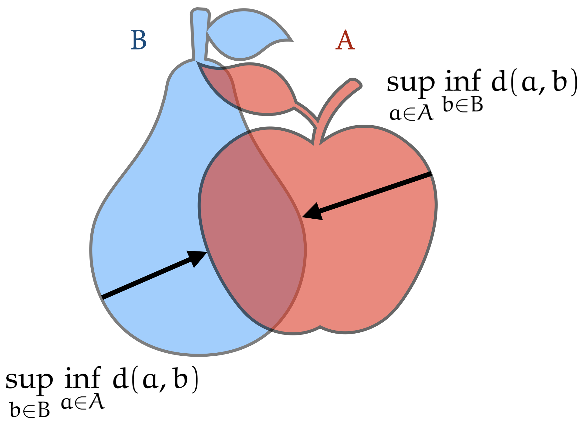
Illustration of Hausdorff distance
The notation may frighten you, but if you break it down into parts, you will find it very intuitive. Part \(\inf_{b\in B} d(a, b)\) means the smallest distance from point \(a\) to any point from set \(B\). Likewise, \(\sup_{a\in A} \inf_{b\in B} d(a, b)\) is the distance of the most distant point from set \(A\). The distance must be symmetric, so in the formula \(d_H(A, B)\), we take the maximum from the value calculated in this way for set \(A\) with respect to set \(B\) and vice versa.
2.3.3 Cauchy sequence
Dear Reader, as you may have already noticed, when constructing fractals, we repeat specific steps over and over again. There is a suggestion here and there that this should be done infinitely many times. However, playing around with infinity is risky, especially if we don’t have guarantees that our calculations will converge somewhere. Where to find those guarantees?
Definition (Cauchy sequence). Cauchy sequence is a sequence of points \(a_n\), such that for any number \(\varepsilon\) greater than zero, one can find such an element \(a_N\) in the sequence that the distance between all subsequent elements is less than \(\varepsilon\).
\[ \forall_{\varepsilon >0} \exists_N \forall_{m,n>N} d(a_m,a_n) \leq \varepsilon. \]
2.3.4 Complete space
Convergent sequences satisfy the Cauchy condition, but there are spaces in which Cauchy sequences do not converge. These are not decent spaces, so we will continue to operate only on decent spaces, i.e., complete spaces.
Definition (complete space). A metric space \((X,d)\) is complete if every Cauchy sequence \(a_n \subset X\) converges in \(X\).
And these are the guarantees of `decency’ that we need.
2.3.5 Contraction
We have a decent space, now let’s talk about transformations. To construct fractals, we can use specific transformations that bring points together. We’ll call them contraction mappings, or contractions for short.
Definition (contraction). A transformation \(T\) is a contraction mapping (contraction) if there is a constant \(\lambda < 1\) such that
\[ \forall_{x,y} d(T(x), T(y)) \leq \lambda d(x,y). \]
That is, for any two points, \(x\) i \(y\), after the transformation, they are closer than before by a scale factor \(\lambda < 1\).
In the examples discussed at the beginning of the chapter, every transformation shown was a contraction. Why? The transformations consisted of rotations, shifting, and scaling. Rotation and shifting do not change the distance between points. And all scaling was done by a factor of less than 1 for each axis.
2.3.6 Affine transformation
Contractions are a very broad class of transformations. We restrict ourselves to a much narrower class of linear transformations with shifts - so-called affine transformations.
An affine transformation is a composition of scaling, rotating, and shifting.
If scaling reduces the figure, such an affine transformation is a contraction since rotation and shifting do not change the distance.
Affine transformations can be easily described in algebraic form as the multiplication of a point by a transformation matrix. This will allow us to shorten the notation of the code that generates the fractal:
\[ T_{rotate, \alpha}(x) = \begin{bmatrix} \cos(\alpha) & -\sin(\alpha) \\ \sin(\alpha) & \cos(\alpha) \end{bmatrix} x, \]
\[ T_{scale, a, b}(x) = \begin{bmatrix} a & 0 \\ 0 & b \end{bmatrix} x, \]
\[ T_{shift, a, b}(x) = x + \begin{bmatrix} a \\ b \end{bmatrix}. \]
2.3.7 Hutchinson’s theorem
At this point someone will say: “OK, each of the transformations is a contraction, but must their composition also be a contraction?”. When constructing the Sierpiński triangle, we admittedly reduced the figure, but then copied it three times. It turns out that the sum of contractions is also a contraction - and this is exactly what Hutchinson’s theorem says.
Hutchinson’s theorem. A transformation \(T = T_1 \cup T_2 \cup ... \cup T_k\) is a contraction if all transformations \(T_1, ..., T_k\) used to define the transformation \(T\) are contractions.
The proof of this claim is not long, it can be found, for example, in Delta of July 2011 [Kici11].
2.3.8 Banach’s fixed point theorem
We already have everything we needed to show Banach’s fixed point theorem, that is, a decent space with a decent distance, in which we use the operator \(T\), which is a contraction. More precisely:
Banach’s fixed point theorem. If \((X, d)\) is a complete metric space, and \(T: X\to X\) is a contraction, then \(T\) has exactly one fixed point \(x\in X\).
The fixed point of the transformation \(T\) is \(x\) such that \(T(x) = x\).
Banach presented the proof of this theorem in his doctoral thesis. It is not very complicated and can be found, for example, in Delta of July 2011 [Kici11]. Here we will limit ourselves only to showing how to look for this fixed point.
Well, it turns out that for any point \(x\) of the space \(X\) the sequence \(T^n(x)\) converges to a fixed point, where \(T^n(x)\) denotes the \(n\)-folded composition of the transformation \(T\), that is, \(T(T(T(...T(x)...)))\). Thus, it is enough to infinitely compose the contractions to find their fixed point.
And such a fixed point are the fractals we construct…