3.6 Examples in Julia
3.6.1 The Sierpinski triangle once again
The following code reproduces the Sierpiński triangle construction presented in this chapter. In the triangle matrix, we define the three vertices of the triangle, and in the point object we put the coordinates of the starting point for the fractal construction. We then move the point toward a random vertex in a loop.
- \(x' = x/2\), \(y' = y/2\) (left corner)
- \(x' = x/2 + \frac 12\), \(y' = y/2\) (right corner)
- \(x' = x/2 + \frac 14\), \(y' = y/2 + \frac{\sqrt{3}}2\) (upper corner)
using Plots

# Number of steps, triangle vertices and colors for transformation.
N = 100000
triangle = [0 0; 0.5 2; 1.5 0.5]
col = ["red" "green" "blue"]
point = [0.1 0]

# Matrix for consecutive points of the Sierpiński triangle.
points = zeros(N, 2)
cols = String[]

# The cols vector collects the colors corresponding to the chosen transformations
# and the coords array collects the pen coordinates after each jump.
for i in 1:N
  ind = rand(1:3,1)
  append!(cols, col[ind])
  point = (point + triangle[ind, :])/2
  coords[i,:] = point
end

scatter(coords[:,1], coords[:,2], color=cols,
        legend=:false, markersize=2, axis=nothing)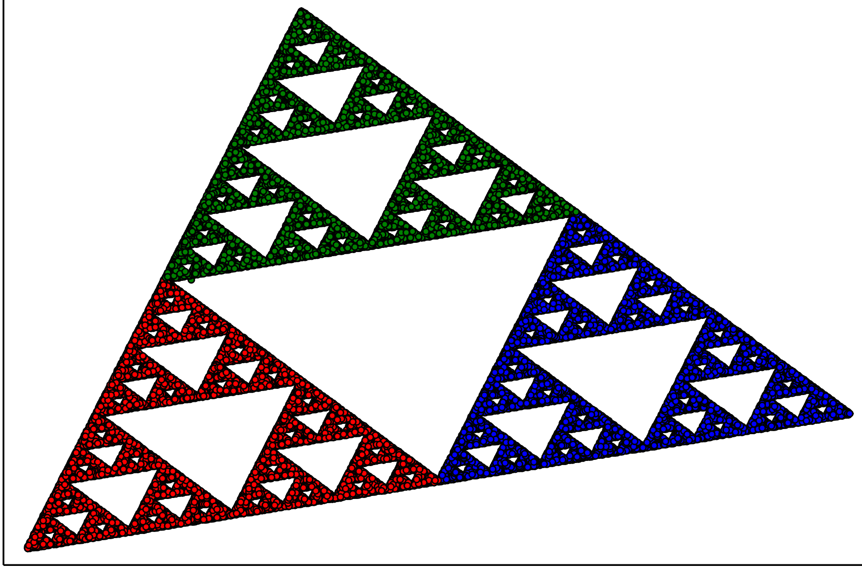
3.6.2 Barnsley fern
using StatsBase

# The following transformations are written as separate functions
# that will later make up the vector of trans.
trans1(x) = [   0.   0.; 0.    0.16]*x
trans2(x) = [0.85  0.04; -0.04 0.85]*x + [0; 1.6]
trans3(x) = [0.2  -0.26;  0.23 0.22]*x + [0; 0.8]
trans4(x) = [-0.15 0.28;  0.26 0.24]*x + [0; 0.44]
trans = [trans1, trans2, trans3, trans4]
point = [0 0]'

col = ["red" "green" "blue" "orange"]
probs = [0.01, 0.79, 0.1, 0.1]

N = 200000
coords = zeros(N, 2)
cols = String[]

for i in 1:N
  # We randomly choose transformations using a vector of *probs* with the frequencies of each transformation.
  # The sample function is available in the StatsBase library.
  ind = sample(1:length(probs), Weights(probs))
  selected_trans = trans[ind[1]]
  point = selected_trans(point)
  coords[i,:] = point
  push!(cols, col[ind])
end

scatter(coords[:,1], coords[:,2], color=cols,
      legend=:false, markersize=1, axis=nothing,
      markerstrokecolor=cols)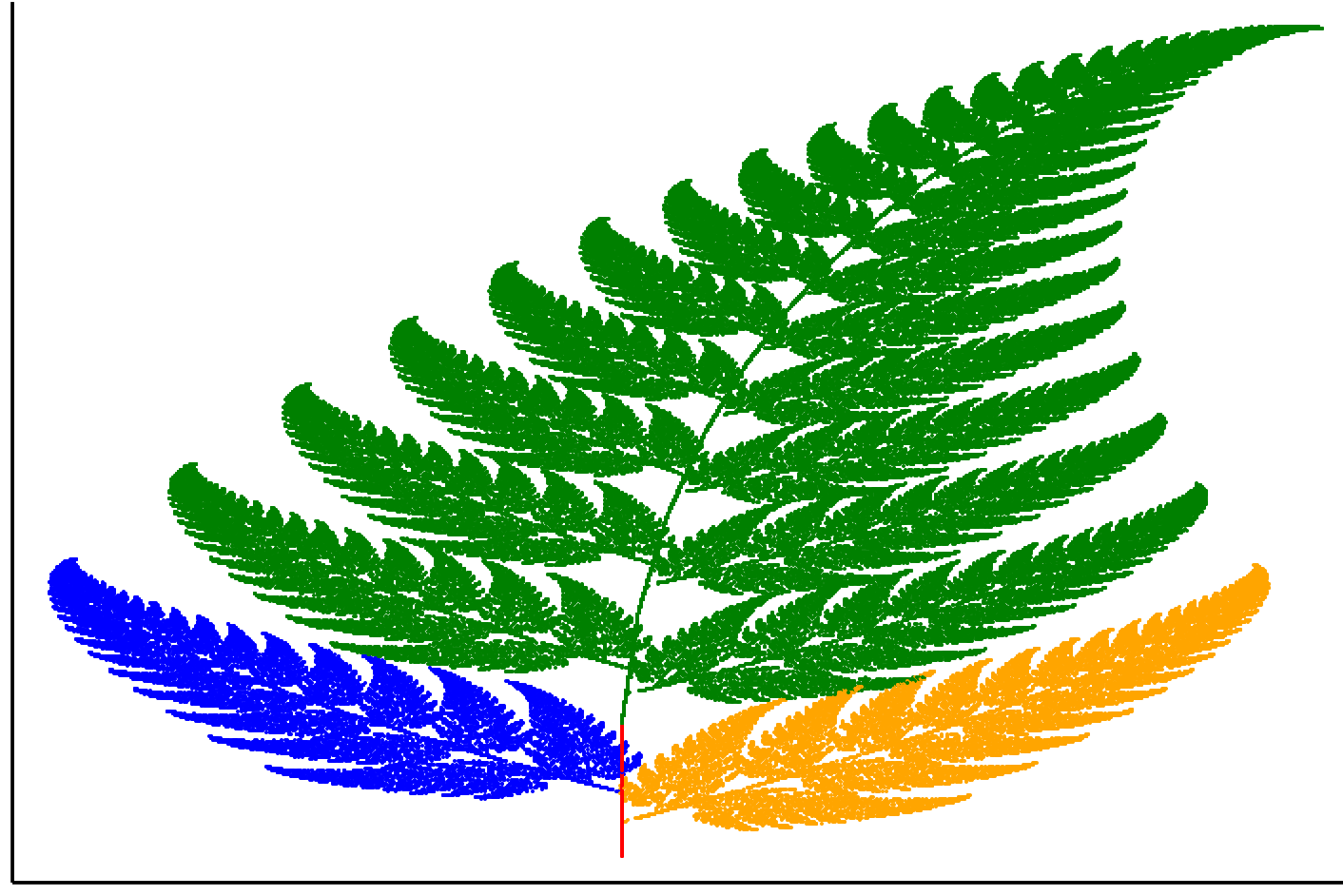
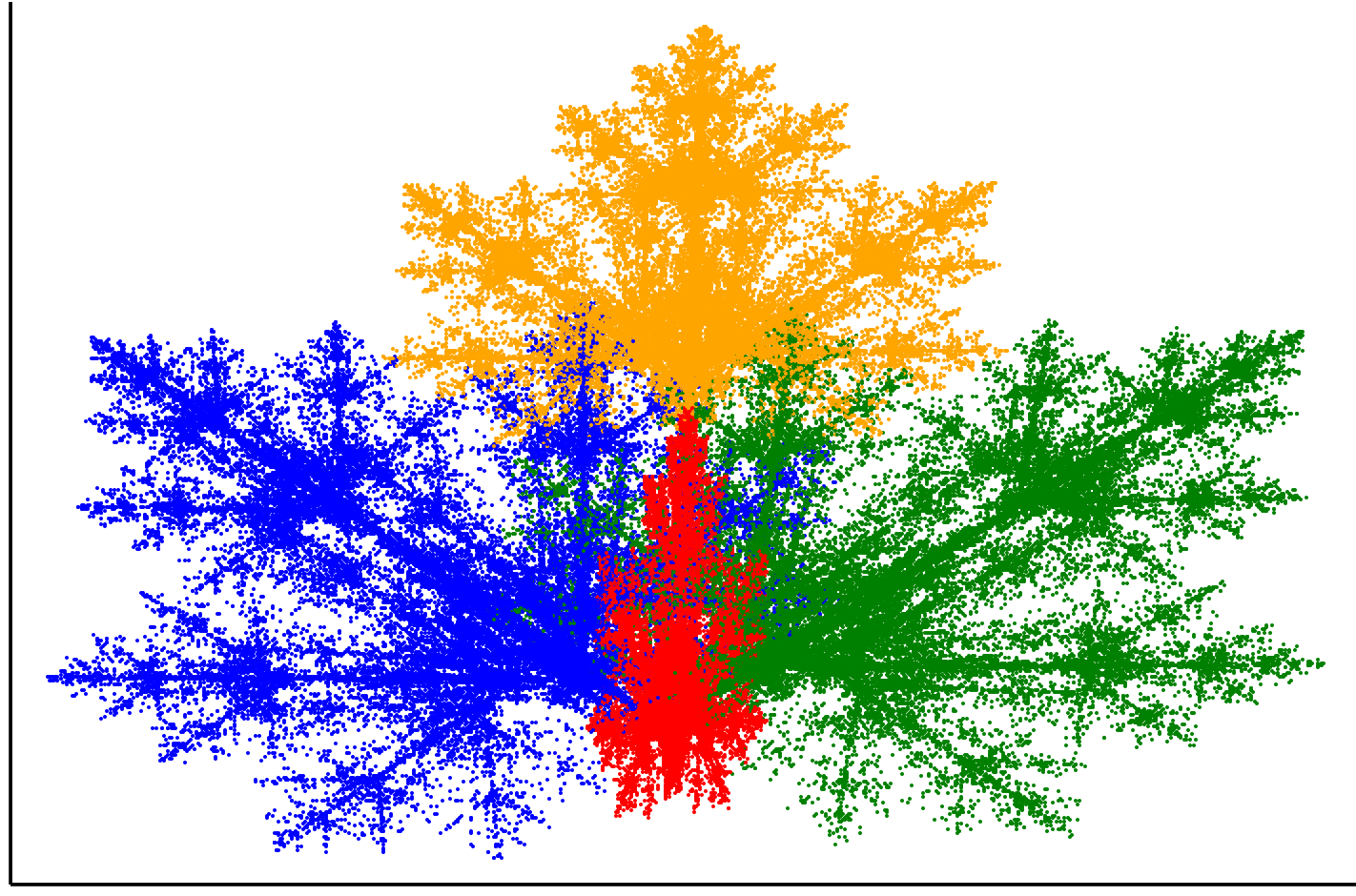
3.6.3 Maple leaf
# We write the transformations as 3x3 matrices representing linear
# transformations. This makes the notation more concise.
affines = [[0.14  0.01  -0.08; 0.0  0.51  -1.31; 0 0 1],
      [0.43   0.52   1.49; -0.45  0.5  -0.75 ; 0 0 1],
      [0.45  -0.49  -1.62;  0.47  0.47  -0.74; 0 0 1],
      [0.49   0.0    0.02;  0.0   0.51  1.62 ; 0 0 1]]
probs = [0.25, 0.25, 0.25, 0.25]
col = ["red", "green", "blue", "orange"]

N = 200000
point = [0 0 1]'
coords = zeros(N, 2)
cols = String[]

for i in 1:N
  # Unlike in the previous chapters, here we do not use recursion.
  # We iteratively count the positions for N jumps and then
  # draw all the determined points with a single scatter instruction.
  ind = sample(1:length(probs), Weights(probs))
  point = affines[ind[1]] * point
  coords[i,:] = point[1:2]
  push!(cols, col[ind])
end

scatter(coords[:,1], coords[:,2], color=cols,
  legend=:false, markersize=1, axis=nothing,
  markerstrokecolor=cols)