1.6 Examples in Julia
When creating fractals, certain operations must be repeated infinitely many times, or at least for a very long time. Efficient, flexible, and very very fast programming languages are great for this. Julia is such a language. It can be downloaded from https://julialang.org/.
Here is some information to help you understand the following examples.
- The following examples use the
Plotslibrary, a basic library for the Julia language. Theplot()function from this library creates an empty graph. You can add more figures to it with theplot!()function. In the examples below, we will create additional filled polygons, triangles, and squares in this way. - Julia is a language very friendly to mathematical operations, you can use mathematical functions such as
sqrt()without additional modules. Arithmetic operators such as+or/work for both numbers and vectors. - To make the code more readable, we use recursion, that is, a construction in which a function calls itself. New functions are defined using the word
function. You can use a simplified definition with the=operator for shorter functions. We will use the shorter way when defining functionsline,triangle,square.
1.6.1 Cantor dust
Let’s start drawing fractals with Cantor dust. For this, we will use the recursive function dust, which takes three arguments: x – the beginning of the fractal, scale -- the size of the fractal, anddepth` – the current nesting level of the fractal.
# Package with graphics functions.
using Plots

# Function that defines a line segment.
line(x, scale) = Shape([x, x+scale], [0, 0])

# Rekurencyjna funkcja do rysowania kurzu.
# Recursive function to draw dust.
# If depth=1, it draws a line segment,
# if depth>1 it draws two copies of Cantor dust side by side.
function dust(x, scale, depth=1)
    if depth == 0
        plot!(line(x, scale), color=:black, legend=:false)
    else
      dust(x, scale/3, depth - 1)
      dust(x + scale*2/3, scale/3, depth-1)
    end
end

# Clear the screen and start drawing dust.
plot(0, xlim=(-0.1,1.1), ylim=(-0.1,0.1), axis=nothing)
dust(0.0, 1.0, 4)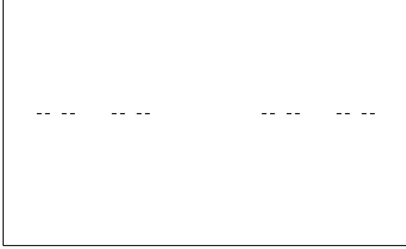
The result of executing the following instructions
1.6.2 Sierpinski triangle
It’s time for the iconic Sierpiński triangle. To draw it, we will use the recursive function sierpinski(), which takes four arguments: x, y – the location from which to draw the fractal, scale – the size of the fractal, and depth depth – the current nesting level of the fractal.
triangle(x, y, scale) = Shape([x, x+scale, x+scale/2, x],
      [y, y, y+scale*sqrt(3)/2, y])

# Recursive function to draw a Sierpiński triangle.
# If depth=1, we draw a triangle using the triangle() function,
# if depth>1, we draw three Sierpiński triangles.
function sierpinski(x, y, scale, depth=1)
  if depth==0
    plot!(triangle(x,y,scale),color=:black,legend=:false)
  else
    sierpinski(x, y, scale/2, depth-1)
    sierpinski(x+scale/2, y, scale/2, depth-1)
    sierpinski(x+scale/4,y+sqrt(3)*scale/4,scale/2,depth-1)
  end
end

plot(0, xlim=(0,1), ylim=(0,1), axis=nothing)
sierpinski(0, 0, 1, 6)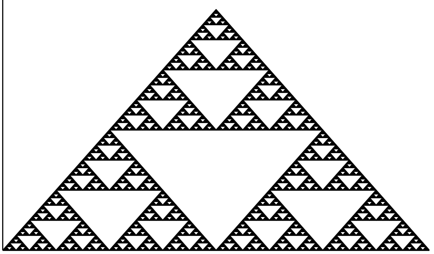
The result of executing the following instructions
1.6.3 Sierpinski carpet
The fractal structure proposed by Wacław Sierpiński can be repeated for other shapes.
square(x, y, w) = Shape([x, x+w, x+w, x], [y, y, y+w, y+w])

# We use the square function defined above to draw a square.
function carpet(x, y, scale, depth=1)
  if depth==0
    plot!(square(x,y,scale), color=:black, legend=:false)
  else
    carpet(x, y, scale/3, depth-1)
    carpet(x, y+scale, scale/3, depth-1)
    carpet(x, y+2scale, scale/3, depth-1)
    carpet(x+scale, y, scale/3, depth-1)
    carpet(x+scale, y+2scale, scale/3, depth-1)
    carpet(x+2scale, y, scale/3, depth-1)
    carpet(x+2scale, y+scale, scale/3, depth-1)
    carpet(x+2scale, y+2scale, scale/3, depth-1)
  end
end

plot(0, xlim=(0,3), ylim=(0,3), axis=nothing)
carpet(0.0, 0.0, 1.0, 5)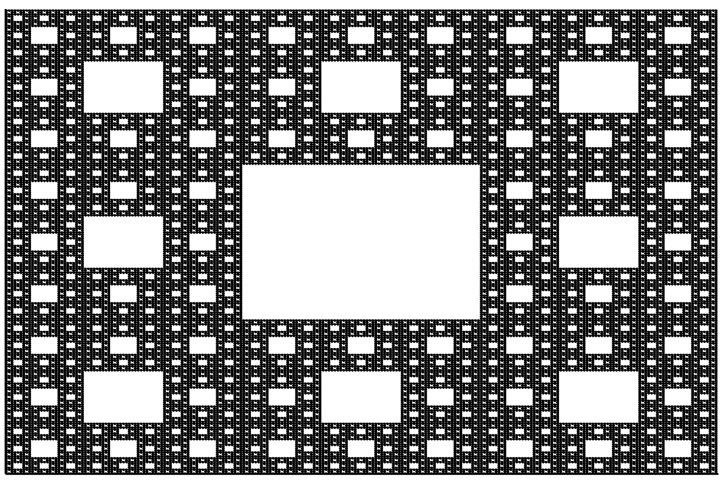
The result of executing the following instructions