2.6 Examples in Julia

2.6.1 Sierpinski triangle

We can build fractals from ordinary dots, we do not need more sophisticated figures. The following example builds a Sierpiński triangle from dots.

The following program repeats the sierpinski depth function composition a number of times. In theory, we would do this indefinitely, but it only takes a few steps to get a clear picture. The number of points grows exponentially, so after \(k\) steps it’s equal to \(3^k\)

using Plots

function sierpinski(x, y, depth) 
  if depth > 1 
    sierpinski(x/2, y/2, depth-1)
    sierpinski(x/2 + 0.5, y/2, depth-1)
    sierpinski(x/2 + 0.25, y/2 + 0.5, depth-1)
  else
    scatter!([x], [y], color=:black, 
             legend=:false, markersize=2)
  end
end

# Initialize an empty graph and draw Sierpiński triangle.
plot(0, xlim=(-0.1,1.1), ylim=(-0.1,1.1), axis=nothing) 
sierpinski(0, 0, 9)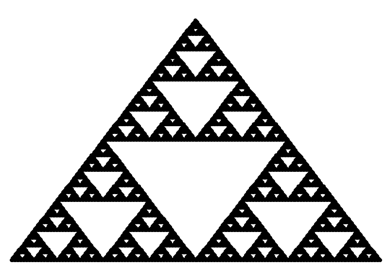

The result of executing the above instructions

2.6.2 Sierpinski pentagon

# Recursively draw each arm of the pentagon.
function pentagon(x, depth, col)
  if depth > 1
    x1 = 0.382x
    x2 = 0.382x + [0.618 0]
    x3 = 0.382x + [0.809 0.588]
    x4 = 0.382x + [0.309 0.951]
    x5 = 0.382x + [-0.191 0.588]
    pentagon(x1, depth-1, "red")  
    pentagon(x2, depth-1, "blue")
    pentagon(x3, depth-1, "green")
    pentagon(x4, depth-1, "orange")
    pentagon(x5, depth-1, "brown")
  else
    # We draw one point at a time, making the whole fractal creation time-consuming.
    # We will do it better in the next chapter.
    scatter!([x[1]], [x[2]], color=col,    
              legend=:false, markersize=2)
  end
end

plot(0, xlim=(-0.35,1.35), ylim=(-0.1,1.6), axis=nothing)
pentagon([0 0], 6, "black")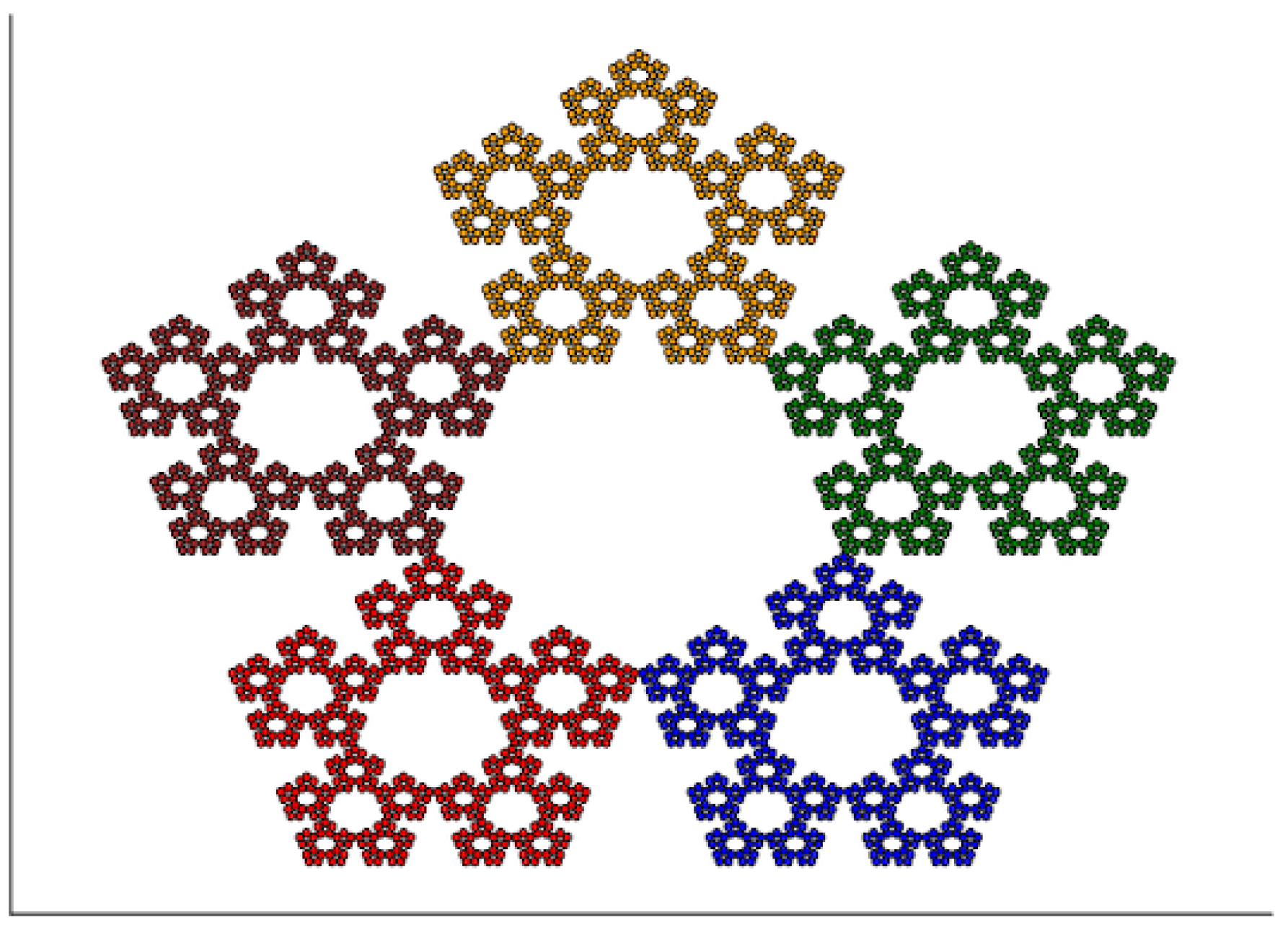

The result of executing the above instructions

2.6.3 Heighway’s Dragon

In the Julia language, matrix addition and scaling are performed using standard operators. We need to define a function for rotating a vector by an angle \(\alpha\).

# Rotate by alpha angle (in degrees).
function rotatex(x, alpha) 
  sa = sin(pi * alpha / 180)
  ca = cos(pi * alpha / 180)
  [ca -sa;  sa ca] * x
end

# Symbol ' stands for matrix transposition. 
# We need it to turn a row vector into a column vector.
function heighway(x, depth, col)
  if depth > 1
    x1 = rotatex(x, -45) * sqrt(0.5)
    x2 = rotatex(x, -135) * sqrt(0.5) + [0.75 0.25]'
    heighway(x1, depth-1, "blue")
    heighway(x2, depth-1, "red")
  else
    scatter!([x[1]], [x[2]], color=col, 
              legend=:false, markersize=2)
  end
end

plot(0, xlim=(-0.5,1.5), ylim=(-1,0.5), axis=nothing)
heighway([0 0]', 14, "black")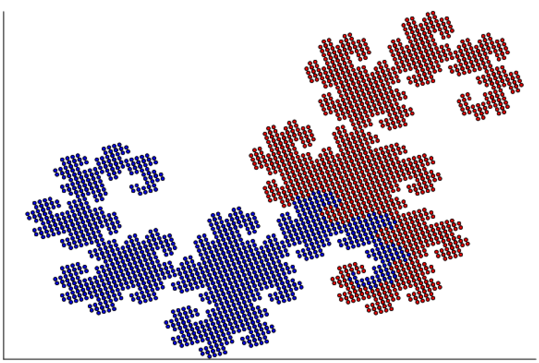

The result of executing the above instructions

2.6.4 Symmetric binary tree / Pythagoras’ tree

The Pythagoras tree construction is very similar to the Heighway dragon. In the last chapter, we will show how to smoothly transition from one to the other.

function sbt(x, depth, col)
  if depth > 1
    x1 = rotatex(x, -45) * 0.7 + [0 1]'
    x2 = rotatex(x, 45)  * 0.7 + [0 1]'
    sbt(x1, depth-1, "blue") 
    sbt(x2, depth-1, "red")
  else
    scatter!([x[1]], [x[2]], color =col, 
              legend=:false, markersize = 2)
  end
end

plot(0, xlim=(-2,2), ylim=(0.5,3), axis=nothing)
sbt([0 0]', 14, "black")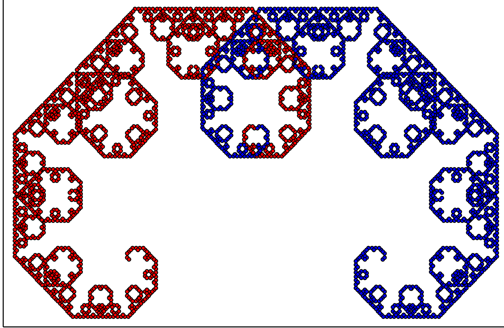

The result of executing the above instructions