3.5 Examples in R
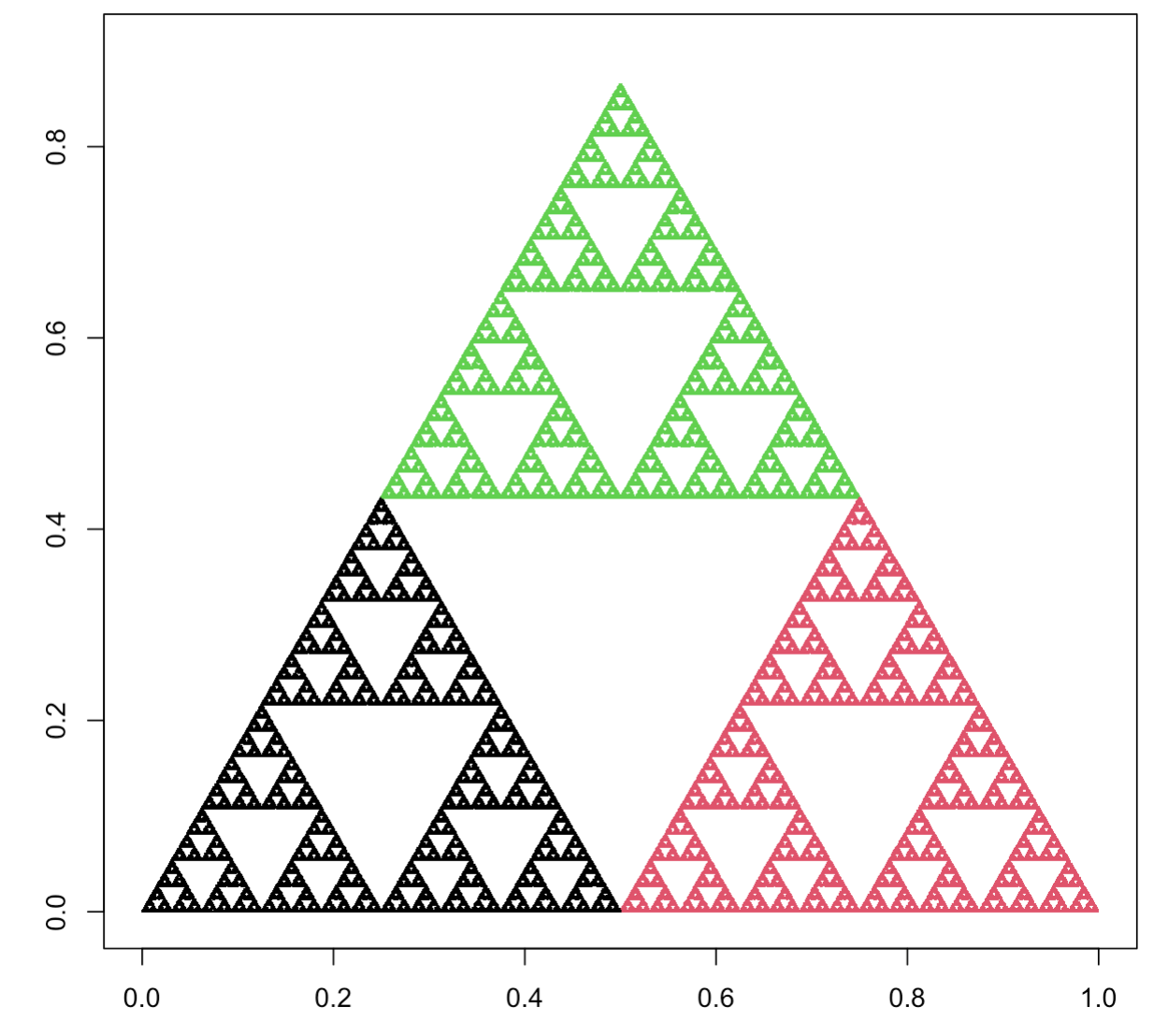
3.5.1 The Sierpinski triangle once again
The following code reproduces the Sierpiński triangle construction presented in this chapter. In the triangle vector, we define the three vertices of the triangle, and in the point object we put the coordinates of the starting point for the fractal construction. We then move the point toward a random vertex in a loop.
- \(x' = x/2\), \(y' = y/2\) (left corner)
- \(x' = x/2 + \frac 12\), \(y' = y/2\) (right corner)
- \(x' = x/2 + \frac 14\), \(y' = y/2 + \frac{\sqrt{3}}2\) (upper corner)
N = 200000
x = y = 0

plot(0, xlim = c(0,1), ylim = c(0,0.9),
     xlab = "", ylab = "", col="white", asp=1)

for (i in 1:N) {
  # We use the three transformations as different scenarios in the switch statement block.
  ind = sample(1:3, 1)
  switch(ind,
         '1' = {x <- x/2; y <- y/2},
         '2' = {x <- x/2 + 1/2; y <- y/2},
         '3' = {x <- x/2 + 1/4; y <- y/2 + sqrt(3)/4})
  points(x, y, pch = ".", col=ind)
}
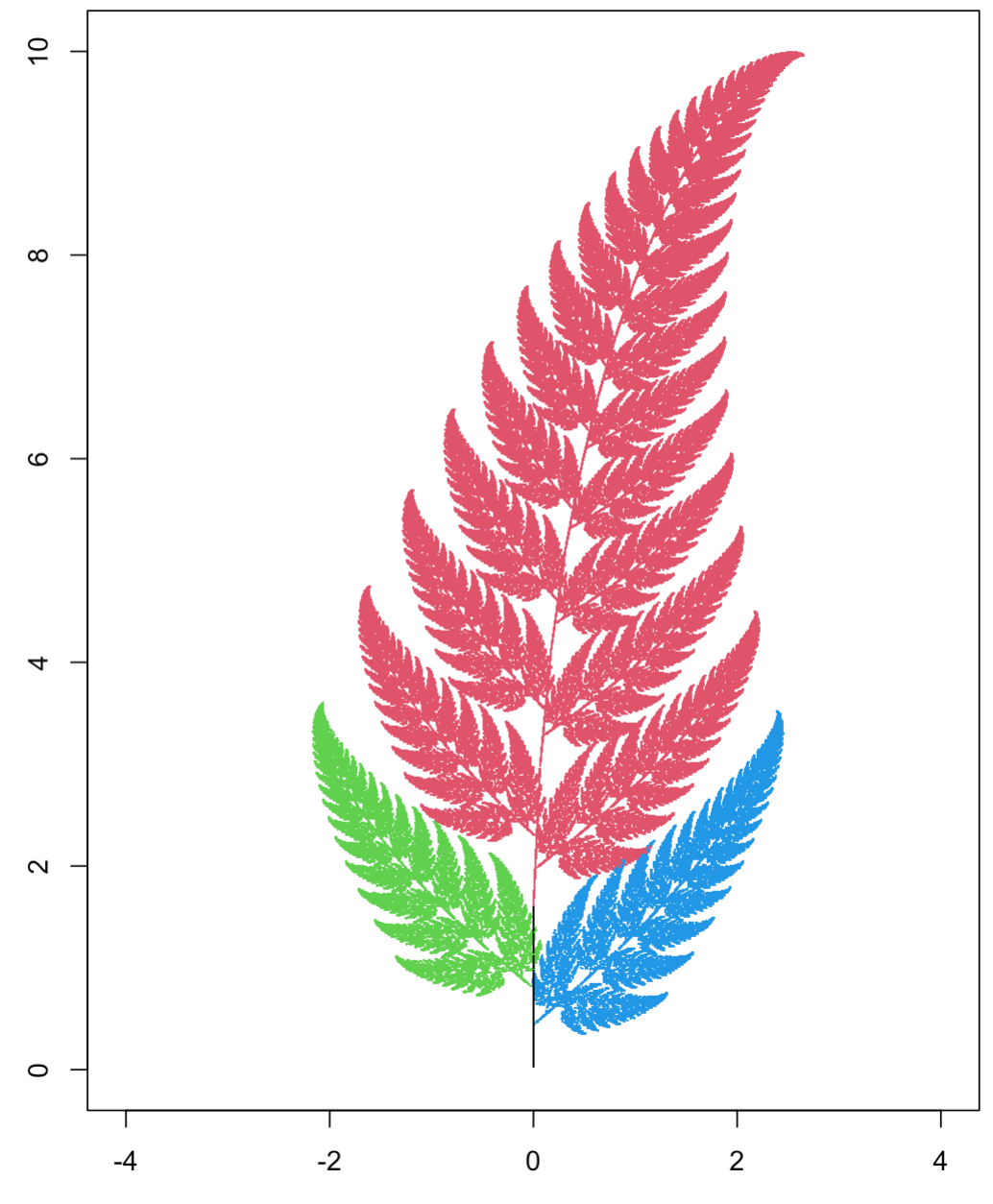
3.5.2 Barnsley fern
trans1 = function(x,y)
   c(0., 0.16*y)
trans2 = function(x,y)
   c(0.85*x + 0.04*y, -0.04*x + 0.85*y + 1.6)
trans3 = function(x,y)
   c(0.2*x - 0.26*y, 0.23*x + 0.22*y + 0.8)
trans4 = function(x,y)
   c(-0.15*x + 0.28*y, 0.26*x + 0.24*y + 0.44)

# In this example, we stored the transformations (which are a function)
# in a list to make it easier to work on them.
trans = list(trans1, trans2, trans3, trans4)
probs = c(0.01, 0.79, 0.1, 0.1)


N = 200000
x = y = 0

plot(0, xlim = c(-2.5,2.5), ylim = c(0,10),
     xlab = "", ylab = "", col="white", asp=1)

for (i in 1:N) {
  ind = sample(seq_along(trans), 1, prob = probs)
  res = trans[[ind]](x, y)
  x = res[1]
  y = res[2]
  points(x, y, pch = ".", col=ind)
}
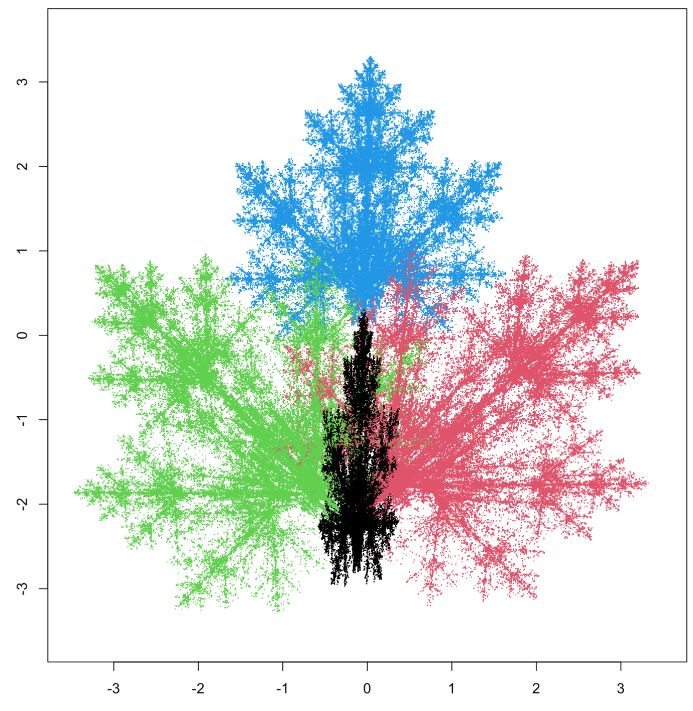
3.5.3 Maple leaf
transform = function(x,y, affine)
  c(affine[1]*x + affine[2]*y + affine[3],
         affine[4]*x + affine[5]*y + affine[6])

N = 400000
x = y = 0

# List of transformations, we store it as a list of vectors of length 6.
affines = list(c(0.14, 0.01, -0.08, 0.0, 0.51, -1.31),
            c(0.43, 0.52, 1.49, -0.45, 0.5, -0.75),
            c(0.45, -0.49, -1.62, 0.47, 0.47, -0.74),
            c(0.49, 0.0, 0.02, 0.0, 0.51, 1.62))
probs = c(0.25, 0.25, 0.25, 0.25)

plot(0, xlim = c(-3.5,3.5), ylim = c(-3.5,3.5),
     xlab = "", ylab = "", col="white", asp=1)

for (i in 1:N) {
  # We randomly choose the transformations with the probabilities
  # indicated in the probs vector.
  ind = sample(seq_along(affines), 1, prob = probs)
  res = transform(x, y, affines[[ind]])
  x = res[1]
  y = res[2]
  points(x, y, pch = ".", col=ind)
}